Voice Recognition with MXNet and Amazon SageMaker

24 minute read

This tutorial will guide you through the necessary steps to build a basic voice recognition service from scratch. We will use a Gluon model with MXNet under the hood. The infrastructure will be based on Amazon SageMaker.

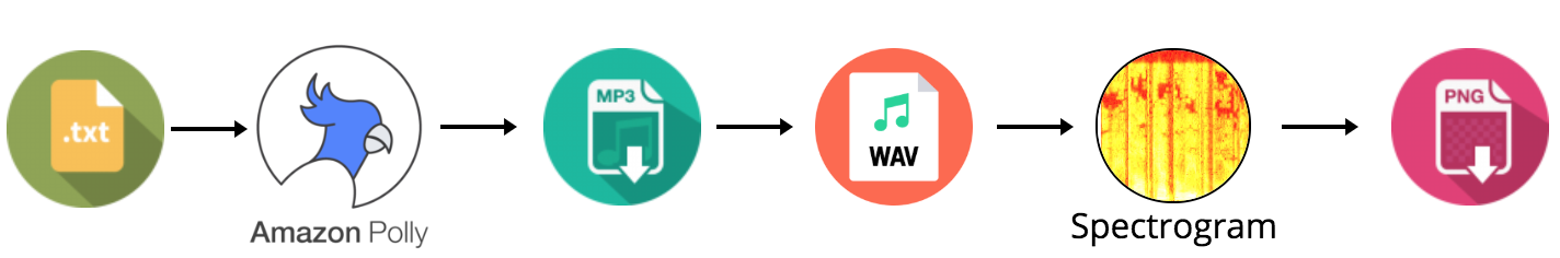
The concrete task at hand is the following: given an English audio recording generated with the help of Amazon Polly, infer which of the eight voices was used for the text-to-speech generation.

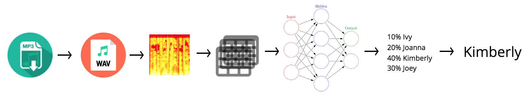
To solve this, I thought of transforming the audio problem to a vision problem. One way to do this is to generate spectrograms of the recordings. The intuition is that the spectrograms contain sufficient information to differentiate between the characteristics of the different voices, from a visual perspective. Naturally, the next step was to employ a neural network containing a number of convolutional layers.

I have started with a trivial architecture thinking that I will probably need to add more capacity very soon. Looking at the different spectrograms, I could see no clear differentiator between them. Surprisingly enough, the simple model I’ve started with did an incredible job at detecting which voices were used in the recordings. To paraphrase Andrej Karpathy, my trivial neural network with two convolutional layers had unreasonable effectiveness.

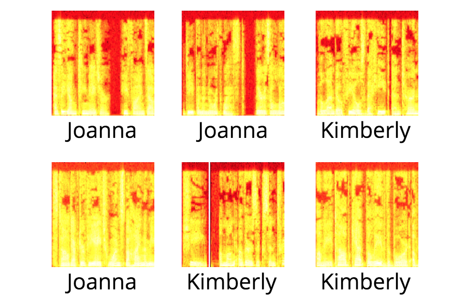
Notice any pattern above? No? Me neither.

Infrastructure

As mentioned in the title, we are going to use Amazon SageMaker to engineer, train and deploy our inference service. You can find basic information on what Amazon SageMaker is and how to use it in one of my previous article here.

After logging in your AWS account, access the Amazon SageMaker console and create a Notebook Instance. For this tutorial, a cheaper ml.m4.xlarge would be appropriate.

Once the instance is operational, open Jupyter and create a new notebook based on the Conda MXNet Python 3 kernel.

The first couple of cells should be used to set-up our Python packages dependencies.

First, install pydub on the notebook instance. pydub is used for converting between .mp3 and .wav.

!pip install pydub > /dev/null

Second, add the rest of the imports.

tarfile is used for working with tar.gz files.
wave is used for getting information about .wav files.
closing is used when working with streams of data.

import random
import base64
import json
import tarfile
import wave
from contextlib import closing
from os import listdir, makedirs
from os.path import isfile, join
from pickle import dump
from sagemaker.mxnet import MXNet
from shutil import rmtree, copy2
from urllib.request import urlretrieve
from tempfile import gettempdir

import boto3
import cv2
import matplotlib
matplotlib.use("agg")
import matplotlib.pyplot as plt
import mxnet as mx
import numpy as np
import pandas as pd
import sagemaker
from pydub import AudioSegment

`matplotlib`

One thing to pay attention to is matplotlib.use("agg"). This is very important because it changes the default matplotlib engine. The reason for that is that the default engine is not easily available on the training instance we are going to use later.

Different engines produce different results. I have spent a few hours trying to understand why the output was different between notebook instance and training instance.

Synthetic Data Generation

For training our model we need a few thousand short sentences. By short sentences I mean sentences that take more than 3 seconds to pronounce, but not more than a few tens of seconds. Actually, the setup I am going to present uses just the first 3 seconds of the recording, but to make it realistic we are going to use some movie review data that we download from Cornell University.

makedirs("data/sentences")

urlretrieve("http://www.cs.cornell.edu/people/pabo/movie-review-data/rotten_imdb.tar.gz",
            "data/sentences/sentences.tar.gz")

Having the raw data downloaded, we will now extract it and save it in one single file for easy reuse. First, we extract the files from the downloaded .tar.gz and then we create two lists from the two files containing sentences. Lastly, we merge the two lists and create a single file with all the sentences. There are 10.000 in total.

tar = tarfile.open("data/sentences/sentences.tar.gz")
tar.extractall("data/sentences")
tar.close()

with open("data/sentences/plot.tok.gt9.5000", "r", encoding = "ISO-8859-1") as first_file:
    first_sentences = first_file.read().split("\n")[0:5000]
with open("data/sentences/quote.tok.gt9.5000", "r", encoding = "ISO-8859-1") as second_file:
    second_sentences = second_file.read().split("\n")[0:5000]

with open("data/sentences/sentences.txt", "w") as sentences_file:
    for sentence in first_sentences + second_sentences:
        sentences_file.write("{}\n".format(sentence))

This how the data/sentences folder should look like now:

> ls data/sentences/
plot.tok.gt9.5000  quote.tok.gt9.5000  sentences.tar.gz
sentences.txt  subjdata.README.1.0

Now we can just create a list of sentences.

with open("data/sentences/sentences.txt", "r", encoding = "ISO-8859-1") as sentences_file:
    sentences = sentences_file.read().split("\n")[:-1]

Moving on to the text-to-speech part provided by Amazon Polly, there are eight voices currently for US English.

voices = ["Ivy", "Joanna", "Joey", "Justin", "Kendra", "Kimberly", "Matthew", "Salli"]

We will now take all the sentences and use them with Amazon Polly to download .mp3 recordings. This will take a while and will cost about 5$.

client = boto3.client("polly")

i = 1

random.seed(42)

makedirs("data/mp3")

for sentence in sentences:
    voice = random.choice(voices)
    file_mask = "data/mp3/sample-{:05}-{}.mp3".format(i, voice)
    i += 1
    response = client.synthesize_speech(
        OutputFormat="mp3",
        Text=sentence,
        TextType="text",
        VoiceId=voice
    )
    with open(file_mask, "wb") as out:
        with closing(response["AudioStream"]) as stream:
            out.write(stream.read())

We now have the .mp3 files which are in essence, our data to work with. Take care of them, as it costs money to regenerate them. Next, we will create a list of these .mp3 files.

This is how the mp3 folder should look like

> ls data/mp3/ | head -10
sample-00001-Matthew.mp3
sample-00002-Joey.mp3
sample-00003-Kendra.mp3
sample-00004-Kimberly.mp3
sample-00005-Kimberly.mp3
sample-00006-Ivy.mp3
sample-00007-Joanna.mp3
sample-00008-Joey.mp3
sample-00009-Joey.mp3
sample-00010-Joey.mp3

Now create a Python list from the files in the mp3 directory.

mp3_files = sorted([f for f in listdir("data/mp3") if isfile(join("data/mp3", f))])

We will now transform the .mp3 files to .wav files so that we can extract the spectrogram from them. Turns out extracting the spectrogram directly from the .mp3 file was pretty difficult, so I just had to make an intermediary conversion to wav. The .wav files we will work with are very small, only 2 seconds.

makedirs("data/wav")

sample_start = random.randint(500, 1000)
sample_finish = sample_start + 2000

for mp3 in mp3_files:
    sound = AudioSegment.from_mp3("data/mp3/{}".format(mp3))[sample_start:sample_finish]
    sound.export("data/wav/{}wav".format(mp3[:-3]), format="wav")

After running this we should have the following listing the wav folder:

> ls data/wav/ | head -10
sample-00001-Matthew.wav
sample-00002-Joey.wav
sample-00003-Kendra.wav
sample-00004-Kimberly.wav
sample-00005-Kimberly.wav
sample-00006-Ivy.wav
sample-00007-Joanna.wav
sample-00008-Joey.wav
sample-00009-Joey.wav
sample-00010-Joey.wav

Again, let’s create a Python list of .wav files:

wav_files = sorted([f for f in listdir("data/wav/") if isfile(join("data/wav/", f))])

Now we need to define a function that given a .wav file, returns its corresponding spectrogram. The .wav file is loaded and frame information is extracted from it. Using matplotlib, a visual representation is constructed. The image is saved to disk.

def graph_spectrogram(wav_file, out):
    wav = wave.open(wav_file, "r")
    frames = wav.readframes(-1)
    sound_info = np.frombuffer(frames, "int16")
    frame_rate = wav.getframerate()
    wav.close()
    fig = plt.figure()
    fig.set_size_inches((1.4, 1.4))
    ax = plt.Axes(fig, [0., 0., 1., 1.])
    ax.set_axis_off()
    fig.add_axes(ax)
    plt.set_cmap("hot")
    plt.specgram(sound_info, Fs=frame_rate)
    plt.savefig(out, format="png")
    plt.close(fig)

We will now use the above function to persist the spectrogram for each of the .wav files:

makedirs("data/spectrograms")

for wav in wav_files:
    graph_spectrogram("data/wav/{}".format(wav), "data/spectrograms/{}png".format(wav[:-3]))

After running the above cell, we should have the following listing in the spectrograms folder:

> ls data/spectrograms/ | head -10
sample-00001-Matthew.png
sample-00002-Joey.png
sample-00003-Kendra.png
sample-00004-Kimberly.png
sample-00005-Kimberly.png
sample-00006-Ivy.png
sample-00007-Joanna.png
sample-00008-Joey.png
sample-00009-Joey.png
sample-00010-Joey.png

As before, we will create a Python list out of the .png files containing the spectrograms:

spectrograms  = sorted([join("data/spectrograms/", f) for f in listdir("data/spectrograms/") if isfile(join("data/spectrograms/", f))])

To make it easier to work with the data, we will now build a pandas data frame containing information about the files we are working with and the labels which need to be attached to the data. The label for the data is extracted from the file name and then converted to the numerical index corresponding to the voices list defined at the beginning of the notebook.

df = pd.DataFrame({
    "wav": [join("data/wav/", f) for f in wav_files],
    "mp3": [join("data/mp3/", f) for f in mp3_files],
    "spectrograms": spectrograms
})
df["label"] = df.spectrogram.str.extract("sample-\d+-(\w+)\.png", expand=False).apply(lambda x: voices.index(x))
df["voice"] = df.spectrogram.str.extract('sample-\d+-(\w+)\.png', expand=False)

A sample from the df pandas data frame looks like this (you’ll have to scroll sideways for this one, sorry):

     mp3                                    spectrogram                                    	wav                                 label    voice
  data/mp3/sample-00001-Matthew.mp3    	data/spectrograms/sample-00001-Matthew.png    	data/wav/sample-00001-Matthew.wav   6        Matthew
  data/mp3/sample-00002-Joey.mp3         data/spectrograms/sample-00002-Joey.png         data/wav/sample-00002-Joey.wav      2        Joey
  data/mp3/sample-00003-Kendra.mp3    	data/spectrograms/sample-00003-Kendra.png    	data/wav/sample-00003-Kendra.wav	4        Kendra
  data/mp3/sample-00004-Kimberly.mp3    	data/spectrograms/sample-00004-Kimberly.png    	data/wav/sample-00004-Kimberly.wav  5        Kimberly
  data/mp3/sample-00005-Kimberly.mp3    	data/spectrograms/sample-00005-Kimberly.png    	data/wav/sample-00005-Kimberly.wav  5        Kimberly

Next thing we do is split the data into training/validation/test datasets. Since this is a classification problem, we want our datasets to be equivalent between them, in other words, they need to have the same proportion of voices used. This is called stratified sampling. The next code cell will do just that. It’s a bit difficult to read, but it will do what it is supposed to .

train = df.groupby("voice").apply(lambda x: x.sample(frac=.8)).reset_index(0, drop=True)
validation = df.loc[~df.index.isin(train.index), :].groupby("voice").apply(lambda x: x.sample(frac=.5)).reset_index(0, drop=True)
test = df.loc[np.logical_not(np.logical_xor(~df.index.isin(train.index), ~df.index.isin(validation.index))), :]

The training dataset contains 80% of the data, the validation and test datasets contain 10% of the data respectively.

A note about train/validation/test datasets

The training dataset will be used for training the model. The validation dataset will be used for improving the model, that is, we want to increase performance on the validation dataset. In production, we will use the model with the highest performance metric on the validation dataset. The test dataset is used just to get a real feel for how the model will perform with unseen data.

Do not use the test dataset for tuning the model. Say you have two models:

Model 1 - validation accuracy: 80% and test accuracy: 90%
Model 2 - validation accuracy: 85% and test accuracy: 87%

You should use Model 2 and discard Model 1. At best, you should try an improve your model so that you end up with a Model 3 - validation accuracy: 86% and test accuracy 88%.

When you are happy with your model structure (architecture), rebuild the model artifact on the whole data. This will be your production model. Many people use in production, the model based on the training dataset, but this is a mistake. Use all the data you have available to build the model. There is no relationship whatsoever between what it means to build the model architecture and what it means to build the model binary. When building the model binary, there is no overfitting problem anymore.

Moving on.

We will now define a function which transforms the .png images and label information into numerical arrays that can be fed into MXNet. The function returns a tuple for the features and dependent variable. This function is explained in more detail further on.

def transform(row):
    img = cv2.imread(row["spectrogram"])
    img = mx.nd.array(img)
    img = img.astype(np.float32)
    img = mx.nd.transpose(img, (2, 0, 1))
    img = img / 255
    label = np.float32(row["label"])
    return img, label

We now execute the function on the pandas data frame to obtain the train and validation NDArray representations.

train_nd = [transform(row) for _, row in train.iterrows()]
validation_nd = [transform(row) for _, row in validation.iterrows()]

Define another function which we will use to serialize numerical arrays to disk into pickles. We will use a temporary location. Since these files can grow quite a lot, it is best to place them where there is a lot of space. On notebook instances, this is the /tmp folder.

def save_to_disk(data, type):
    makedirs("{}/pvdwgmas/data/pickles/{}".format(gettempdir(), type))
    with open("{}/pvdwgmas/data/pickles/{}/data.p".format(gettempdir(), type), "wb") as out:
        dump(data, out)

Use the function to persist the data:

save_to_disk(train_nd, "train")
save_to_disk(validation_nd, "validation")

At this point, we need to initialize an Amazon SageMaker session and use it to upload the data to Amazon S3.

sagemaker_session = sagemaker.Session()

After the data is uploaded to S3, we have the path in the inputs variable.

inputs = sagemaker_session.upload_data(path="{}/pvdwgmas/data/pickles".format(gettempdir()),
                                       bucket="redacted", key_prefix="cosmin/sagemaker/demo")

Lastly, we will create a test folder in which we will keep the test .mp3 files partitioned by their respective voice. This will make it easy for us to test the service at the very end.

makedirs("data/test")
for _, row in test.iterrows():
    makedirs("data/test/{}".format(row["voice"]), exist_ok=True)
    copy2(row["mp3"], "data/test/{}".format(row["voice"]))

Listing the test folder looks like this:

> tree data/test/ -L 1 data/test/
├── Ivy
├── Joanna
├── Joey
├── Justin
├── Kendra
├── Kimberly
├── Matthew
└── Salli

Model Training

Training a model is done on an Amazon SageMaker training instance. For this, the Amazon SageMaker framework requires a script conforming to a predefined interface. With that in mind let’s create a script voice-recognition-sagemaker-script.py

Amazon SageMaker Script - Part I - Training

Training runs in a Docker container based on stripped down image, so some Python packages and functionality which you might expect to find readily available needs to be installed explicitly first. To that extent here is the import list that works out of the box in said Docker container:

import base64
import glob
import json
import logging
import subprocess
import sys
import tarfile
import traceback
import uuid
import wave
from os import unlink, environ, makedirs
from os.path import basename
from pickle import load
from random import randint
from shutil import copy2, rmtree
from urllib.request import urlretrieve

import mxnet as mx
import numpy as np
from mxnet import autograd, nd, gluon
from mxnet.gluon import Trainer
from mxnet.gluon.loss import SoftmaxCrossEntropyLoss
from mxnet.gluon.nn import Conv2D, MaxPool2D, Dropout, Flatten, Dense, Sequential
from mxnet.initializer import Xavier

Now, to install new packages we will define a function:

def install(package):
    subprocess.call([sys.executable, "-m", "pip", "install", package])

With the above function, we will now install a few packages that are not available by default.

install("opencv-python")
install("pydub")
install("matplotlib")

We will now import the installed packages, except for pydub which needs some additional set-up.

import cv2
import matplotlib
matplotlib.use("agg")
import matplotlib.pyplot as plt

You will notice that we have explicitly set the matplotlib engine to be the same as in the Jupyter notebook. This way we can ensure that we have consistent results.

Next are the incantations for making pydub work properly. First, it should be noted that on the Docker container the training script is executed from the /tmp folder so we take advantage of that to set the Docker guest container PATH to include the /tmp folder. We do that so that we can add the ffmpeg and ffprobe binaries which are used by pydub. We essentially do a manual installation of ffmpeg and we make it available in the PATH. The whole procedure involves downloading the latest binary build of ffmpeg, extracting the contents of the installation package to a temporary location and copying the two necessary executables to the /tmp folder, so that they are available in the PATH.

environ["PATH"] += ":/tmp"

rmtree("ffmpeg-tmp", True)
makedirs("ffmpeg-tmp")
urlretrieve("https://johnvansickle.com/ffmpeg/builds/ffmpeg-git-amd64-static.tar.xz",
            "ffmpeg-tmp/ffmpeg-git-64bit-static.tar.xz")

tar = tarfile.open("ffmpeg-tmp/ffmpeg-git-64bit-static.tar.xz")
tar.extractall("ffmpeg-tmp")
tar.close()

for file in [src for src in glob.glob("ffmpeg-tmp/*/**") if basename(src) in ["ffmpeg", "ffprobe"]]:
    copy2(file, ".")
rmtree("ffmpeg-tmp", True)

Having done all of the above, we can now safely include pydub:

from pydub import AudioSegment

We also set the logging options and copy the voices list that we have used in the Jupyter notebook. The voices list will be used for inference, but it is good to have it there already.

logging.basicConfig(level=logging.INFO)

voices = ["Ivy", "Joanna", "Joey", "Justin", "Kendra", "Kimberly", "Matthew", "Salli"]

`train` function

We will now define the train function, which is quite large as compared to everything we have done until now. I am going to break it down into pieces so it is easier to digest.

The function definition looks like this:

def train(hyperparameters, channel_input_dirs, num_gpus, hosts):

First we read the hyperparameters that we will use for the model:

batch_size = hyperparameters.get("batch_size", 64)
epochs = hyperparameters.get("epochs", 3)

We lock the random seed into place so that we can get consistent results:

mx.random.seed(42)

The Amazon SageMaker framework conveniently copies for us the train/validation datasets from S3 to the training instance. The location of the data can be fetched like this:

training_dir = channel_input_dirs["training"]

We now takes the pickle files and load the NDArrays stored within them:

with open("{}/train/data.p".format(training_dir), "rb") as pickle:
    train_nd = load(pickle)
with open("{}/validation/data.p".format(training_dir), "rb") as pickle:
    validation_nd = load(pickle)

Having the NDArrays in place, we use the Gluon DataLoader classes to iterate through the data while training.

train_data = gluon.data.DataLoader(train_nd, batch_size, shuffle=True)
validation_data = gluon.data.DataLoader(validation_nd, batch_size, shuffle=True)

The model

Now is time to define the neural network. Behold the complexity:

net = Sequential()
with net.name_scope():
    net.add(Conv2D(channels=32, kernel_size=(3, 3), padding=0, activation="relu"))
    net.add(Conv2D(channels=32, kernel_size=(3, 3), padding=0, activation="relu"))
    net.add(MaxPool2D(pool_size=(2, 2)))
    net.add(Dropout(.25))
    net.add(Flatten())
    net.add(Dense(8))

The last layer is a dense layer of 8 neurons corresponding to the 8 voices.

After the excruciating process of designing the neural network architecture, we need to set the context in which data will be processed: CPU or GPU.

ctx = mx.gpu() if num_gpus > 0 else mx.cpu()

Training a neural network is easier if we start with decent values for the parameters. For this purpose, we use the Xavier initializer.

net.collect_params().initialize(Xavier(magnitude=2.24), ctx=ctx)

Since we have a classification problem, we will use the cross-entropy for the loss function.

loss = SoftmaxCrossEntropyLoss()

The next part is for when you want to have distributed training. I have not used it for this particular task, but I think it is good practice to have it in there for the case when you want to use distributed training.

if len(hosts) == 1:
    kvstore = "device" if num_gpus > 0 else "local"
else:
    kvstore = "dist_device_sync'" if num_gpus > 0 else "dist_sync"

The trainer will use the adam optimizer. MXNet features some interesting optimizers in its latest version, you might want to check that as well.

trainer = Trainer(net.collect_params(), optimizer="adam", kvstore=kvstore)

As stated on other occasions, training is not nice. This has to change and will be probably done, but for now, we will rely on the autograd function to almost manually do backpropagation. Here it goes.

smoothing_constant = .01

for e in range(epochs):
    moving_loss = 0
    for i, (data, label) in enumerate(train_data):
        data = data.as_in_context(ctx)
        label = label.as_in_context(ctx)
        with autograd.record():
            output = net(data)
            loss_result = loss(output, label)
        loss_result.backward()
        trainer.step(batch_size)

        curr_loss = nd.mean(loss_result).asscalar()
        moving_loss = (curr_loss if ((i == 0) and (e == 0))
                       else (1 - smoothing_constant) * moving_loss + smoothing_constant * curr_loss)

    validation_accuracy = measure_performance(net, ctx, validation_data)
    train_accuracy = measure_performance(net, ctx, train_data)
    print("Epoch %s. Loss: %s, Train_acc %s, Test_acc %s" % (e, moving_loss, train_accuracy, validation_accuracy))

What the code does is that it trains on batches and it manually calls backpropagation to minimize the loss function. There is also some logging attached so that you can see progress. The logging part makes use of a measure_performance function, which calculates accuracy. The function essentially runs inference with the current version of the model on batches of data.

def measure_performance(model, ctx, data_iter):
    acc = mx.metric.Accuracy()
    for _, (data, labels) in enumerate(data_iter):
        data = data.as_in_context(ctx)
        labels = labels.as_in_context(ctx)
        output = model(data)
        predictions = nd.argmax(output, axis=1)
        acc.update(preds=predictions, labels=labels)
    return acc.get()[1]

The last thing the train function does is return the neural network model. This is important because then the model is saved and persisted to Amazon S3 as an artifact.

return net

`save` function

The training part of the script only needs the save function. This function receives as input the model returned by the train function and saves it to disk.

def save(net, model_dir):
    y = net(mx.sym.var("data"))
    y.save("{}/model.json".format(model_dir))
    net.collect_params().save("{}/model.params".format(model_dir))

The Amazon SageMaker script file should now look similar to this gist .

Initialising Training

Going back to the Jupyter notebook we can start training. For this purpose, we will create an Amazon SageMaker MXNet estimator. Most of the parameters are self explanatory. The role is the Amazon IAM role used for permissions. The py_version indicates that all code is Python 3.x and not 2.x which is the default. The framework_version indicates which version of MXNet is used for training.

estimator = MXNet("voice-recognition-sagemaker-script.py",
          role=sagemaker.get_execution_role(),
          train_instance_count=1,
          train_instance_type="ml.p2.xlarge",
          hyperparameters={"epochs": 5},
          py_version="py3",
          framework_version="1.1.0")

Triggering training is only a matter of calling the fit method:

estimator.fit(inputs)

This will take some time, as in about 10 minutes, and will cost a few cents. Towards the end of the long listing that gets printed you will be able to see the logging part we have added in the train function:

Epoch 0. Loss: 1.19020674213, Train_acc 0.927615951994, Test_acc 0.924924924925
Epoch 1. Loss: 0.0955917794597, Train_acc 0.910488811101, Test_acc 0.904904904905
Epoch 2. Loss: 0.0780380586131, Train_acc 0.982872859107, Test_acc 0.967967967968
Epoch 3. Loss: 0.0515212092374, Train_acc 0.987123390424, Test_acc 0.95995995996
Epoch 4. Loss: 0.0513322874282, Train_acc 0.995874484311, Test_acc 0.978978978979
===== Job Complete =====
Billable seconds: 337

This looks pretty good. We now have a solid model and its corresponding artifact has been persisted to S3.

Amazon SageMaker Script - Part II - Deployment

For deploying the model as a service we will have to go back to the voice-recognition-sagemaker-script.py and add the necessary functions that are expected by the Amazon SageMaker framework.

`model_fn` function

The first function we need to add is the one used for loading the model into memory from disk.

def model_fn(model_dir):
    with open("{}/model.json".format(model_dir), "r") as model_file:
        model_json = model_file.read()
    outputs = mx.sym.load_json(model_json)
    inputs = mx.sym.var("data")
    param_dict = gluon.ParameterDict("model_")
    net = gluon.SymbolBlock(outputs, inputs, param_dict)
    # We will serve the model on CPU
    net.load_params("{}/model.params".format(model_dir), ctx=mx.cpu())
    return net

This is essentially the reverse of the save method. One important thing to note is the computation context used. You can use either CPU or GPU depending on the type of machine you use for serving. If it has only CPU capabilities, you have to use the mx.cpu() context, otherwise you can use both (preferably mx.gpu()).

The function returns the loaded model.

`transform_fn` function

This is a big function that serves several purposes. It is responsible for:

accepting input
decoding the input
running the inference
encoding the output
returning the output

Amazon SageMaker is supposed to be able to run all of these functionalities as separate functions, which is definitely a better practice. For this tutorial, however, I have chosen the easy path of having just one function. This is also because I have had a bad experience trying to make the individual functions work in my previous MXNet tutorial. I would probably be more successful now since Amazon has open sourced the MXNet Model Server and related Docker containers.

Before I present the actual transform_fn method, there are some utility functions that need to be introduced first.

`mpeg2file`

This function accepts as input a binary representation of, well actually anything, and writes it to disk. The function is generic but we will only use it to persist .mp3 files received by the inference service.

def mpeg2file(input_data):
    mpeg_file = "{}.mp3".format(str(uuid.uuid4()))
    with open(mpeg_file, "wb") as fp:
        fp.write(input_data)
    return mpeg_file

`mpeg2wav`

This function loads a .mp3 file, samples 2 seconds from it and saves it as a .wav file. The .mp3 file is deleted, and the name of the .wav file is returned.

def mpeg2wav(mpeg_file):
    sample_start = randint(500, 1000)
    sample_finish = sample_start + 2000
    sound = AudioSegment.from_mp3(mpeg_file)[sample_start:sample_finish]
    wav_file = "{}.wav".format(str(uuid.uuid4()))
    sound.export(wav_file, format="wav")
    unlink(mpeg_file)
    return wav_file

`wav2img`

This function loads a .wav file and generates the spectrogram from it. The spectrogram is saved as .png file. This is the function where matplotlib is used and where it is important to use the same engine as in the data engineering part in the Jupyter notebook.

Load the audio file using a dedicated library for working with .wav files.
Extract frame information from the audio file.
Using matplotlib create a visual representation of the spectrogram.
The spectrogram is saved to disk.
The audio file is removed from the disk.
The name of the .png file is returned.

def wav2img(wav_file):
    wav = wave.open(wav_file, "r")
    frames = wav.readframes(-1)
    sound_info = np.frombuffer(frames, "int16")
    frame_rate = wav.getframerate()
    wav.close()
    fig = plt.figure()
    fig.set_size_inches((1.4, 1.4))
    ax = plt.Axes(fig, [0., 0., 1., 1.])
    ax.set_axis_off()
    fig.add_axes(ax)
    plt.set_cmap("hot")
    plt.specgram(sound_info, Fs=frame_rate)
    img_file = "{}.png".format(str(uuid.uuid4()))
    plt.savefig(img_file, format="png")
    plt.close(fig)
    unlink(wav_file)
    return img_file

`img2arr`

This function simply transforms an image into its normalized numerical representation.

Using the computer vision library load the .png file corresponding to the input file name.
Convert the numpy array to an MXNet NDArray,
Cast the numerical values to the appropriate type.
Reshape the array so that it matches the structure that MXNet expects.
Normalise the numerical values.
Convert back to numpy so that the output can easily be adjusted after it is returned.
Add another level to the root of the array shape. This is so that a single image can be interpreted as a batch.
Remove the image file from disk.

def img2arr(img_file):
    img = cv2.imread(img_file)
    img = mx.nd.array(img)
    img = img.astype(np.float32)
    img = mx.nd.transpose(img, (2, 0, 1))
    img = img / 255
    img = img.asnumpy()
    img = np.expand_dims(img, axis=0)
    unlink(img_file)
    return img

Now, the transform_fn function has two ways of working. It can accept a single mp3 and infer the voice that was used, or it can accept a batch of mp3 and will return an array of voices used, corresponding respectively to the received mp3 files.

I’m first going to illustrate how inference works for one single mp3. The transform_fn uses the content_type parameter to decide on which type of inference it should execute.

The audio binary data must be sent base64 encoded and naturally, it needs to be decoded on our side. We then apply in order the functions to:

Save the input data as an mp3.
Save the mp3 as wav.
Extract the spectrogram representation from the .wav and save it as a .png.
Extract the numpy representation of the image.
Convert the numpy representation to an MXNet NDArray representation.
Use the NDArray as input for the model and get the predictions
Since this is a classification problem, what is returned is a list of probabilities for the 8 voices used. We are only interested in the index of the highest probability, so the index of maximum value.
Return a JSON with the literal name of the inferred voice.

def transform_fn(model, input_data, content_type, accept):
    if content_type == "audio/mp3" or content_type == "audio/mpeg":
        mpeg_file = mpeg2file(base64.b64decode(input_data))
        wav_file = mpeg2wav(mpeg_file)
        img_file = wav2img(wav_file)
        np_arr = img2arr(img_file)
        mx_arr = mx.nd.array(np_arr)
        logging.info(mx_arr.shape)
        logging.info(mx_arr)
        response = model(mx_arr)
        response = nd.argmax(response, axis=1) \
            .asnumpy() \
            .astype(np.int) \
            .ravel() \
            .tolist()[0]
        return json.dumps(voices[response]), accept
    else:
        raise ValueError("Cannot decode input to the prediction.")

At this point, we have everything we need for a fully functional inferring service, but let’s also add the batch mode functionality. We just need to add an elif to the function.

Unsurprisingly, the idea is the same. We use the same function as before, in the same sequence, but we apply them at the list level. Perhaps the only line that needs more explaining is np_arr = np.concatenate(np_arrs) which takes the individual numpy arrays for each of the mp3 in the payload, and concatenates them into one big array, the batch.

    elif content_type == "application/json":
        json_array = json.loads(input_data, encoding="utf-8")
        mpeg_files = [mpeg2file(base64.b64decode(base64audio)) for base64audio in json_array]
        wav_files = [mpeg2wav(mpeg_file) for mpeg_file in mpeg_files]
        img_files = [wav2img(wav_file) for wav_file in wav_files]
        np_arrs = [img2arr(img_file) for img_file in img_files]
        np_arr = np.concatenate(np_arrs)
        nd_arr = nd.array(np_arr)
        response = model(nd_arr)
        response = nd.argmax(response, axis=1) \
            .asnumpy() \
            .astype(np.int) \
            .ravel() \
            .tolist()
        return json.dumps([voices[idx] for idx in response]), accept

We are now done with the voice-recognition-sagemaker-script.py script. The complete listing can be found in this gist.

Back to the Jupyter notebook, we would like to deploy the model we have previously built. Unfortunately, the voice-recognition-sagemaker-script.py script that was packed with the model, did not contain the hosting part. That is because we have trained the model before adding the rest of the functions. Deploying now would simply fail. The best option is to rerun the training job, so basically, execute again the cell with estimator.fit(inputs). You will see the same output as before.

Now, to actually deploy we have to execute this code cell:

predictor = estimator.deploy(instance_type="ml.m4.xlarge", initial_instance_count=1)

We will use just one instance for the service and it will be a CPU based one (remember when we’ve talked about the model_fn function).

The deployment will take a few minutes.

Testing the endpoint

The service should now be up and running so let’s see if it does what it is supposed to.

First, we will test how the service responds to a request with one mp3. You can use the example mp3 from here or you can use Amazon Polly to generate your own audio file. Just make sure you use one of the US English voices. Also, be warned that the inferring endpoint has an upper limit on the payload size so don’t try sending an audiobook.

So what happens here is that we read the .mp3 and we base64 encode it. Then we just send the request to our service endpoint and we specify that there is just one audio/mp3 and we expect a JSON back. Funny enough, for this particular sample, Kimberly gets predicted as Joanna .

with open("Kimberly recites some shameless self promotion ad.mp3", "rb") as audio_file:
    payload = base64.b64encode(audio_file.read()).decode("utf-8")
    response = sagemaker_runtime_client.invoke_endpoint(
        EndpointName=predictor.endpoint,
        Body=payload,
        ContentType="audio/mp3",
        Accept="application/json"
    )["Body"].read()
    print("Kimberly predicted as {}".format(json.loads(response, encoding="utf-8")))

For testing the batch mode, we will rely on the .mp3 files in the data/test folder. Those files have never been seen by the model before. We loop through all the partitioned voices and create small batches of 5 files that we send towards the service. We keep track of what is correct and what we miss and we compute an accuracy for each of the voices. The difference here is that the base64 mp3 are stored in a list and then, when sent, the content type is set to application/json.

for directory in listdir("data/test"):
    batch = []
    cnt = 0
    total = 0
    detected = 0
    for file in listdir("data/test/{}".format(directory)):
        with open("data/test/{}/{}".format(directory, file), "rb") as audio_file:
            batch.append(base64.b64encode(audio_file.read()).decode("utf-8"))
            cnt += 1
            if cnt == 5:
                binary_json = json.dumps(batch).encode("utf-8")
                response = sagemaker_runtime_client.invoke_endpoint(
                    EndpointName=predictor.endpoint,
                    Body=binary_json,
                    ContentType="application/json",
                    Accept="application/json"
                )["Body"].read()
                individual_predictions = json.loads(response, encoding="utf-8")
                for prediction in individual_predictions:
                    total += 1
                    if prediction == directory:
                        detected += 1
                cnt = 0
                batch = []
    print("""Recordings with {}:
        Total: {}
        Detected: {}
        Accuracy: {:0.2f}
    """.format(directory, str(total), str(detected), detected/total))

You should get something similar to this:

Recordings with Salli:
        Total: 125
        Detected: 121
        Accuracy: 0.97

Recordings with Kimberly:
        Total: 120
        Detected: 115
        Accuracy: 0.96
...

We have now finished the tutorial. The full listing for the notebook can be found in this gist.

I have also created a GitHub respository for this, which is probably easier to look at then the above gists.

Cosmin Sanda

Voice Recognition with MXNet and Amazon SageMaker

Infrastructure

`matplotlib`

Synthetic Data Generation

A note about train/validation/test datasets

Model Training

Amazon SageMaker Script - Part I - Training

`train` function

The model

`save` function

Initialising Training

Amazon SageMaker Script - Part II - Deployment

`model_fn` function

`transform_fn` function

`mpeg2file`

`mpeg2wav`

`wav2img`

`img2arr`

Testing the endpoint

Comments

Cosmin Sanda

Infrastructure

matplotlib

Synthetic Data Generation

A note about train/validation/test datasets

Model Training

Amazon SageMaker Script - Part I - Training

train function

The model

save function

Initialising Training

Amazon SageMaker Script - Part II - Deployment

model_fn function

transform_fn function

mpeg2file

mpeg2wav

wav2img

img2arr

Testing the endpoint

Comments

`matplotlib`

`train` function

`save` function

`model_fn` function

`transform_fn` function

`mpeg2file`

`mpeg2wav`

`wav2img`

`img2arr`